Section 12
Recovery with Two-Phase Commit
Suppose a transaction T requires subtxns at sites A, B, C. Site A is the coordinator. Consider the following sequence of events:
-
After the last operation in T, site A
- sends prepare messages to B and C
- puts its own subtransaction in the ready state
-
Sites B and C...
- put their subtransactions in the ready state
- send ready messages to A
-
Site A...
- writes its commit record
- sends commit messages to B and C
-
Site B writes its commit record
-
Site C writes its commit record
Recall that a subtxn can only enter the committed state from the ready state after receiving a commit message.
Now, consider the following scenarios:
-
Suppose C crashes before writing its commit record. What happens?
The last log record for T at C is a ready record, so C must contact A or B to determine whether to commit or to undo T. If C can’t reach another site, it must block. This is the case where the last record in the log is a ready record. -
Suppose B crashes after writing its commit record. What happens?
Redo the transaction as needed. This is the case where the last record in the log is a commit record. -
Suppose B crashes before writing its ready record. What happens?
Undo the transaction as needed. This is the case where the last record in the log is not a ready record and not a commit record. Instead, the last record may be a do-not-commit record or another kind of record from before 2PC began. -
Suppose A crashes before writing its commit record. What happens?
In this case the coordinator fails, and B and C sent ready messages but did not receive a response from the (failed) coordinator. Since neither B nor C has a commit or abort record, both sites must wait until A recovers. -
Suppose A crashes after writing its commit record. What happens?
In this case the coordinator also fails, but A has a commit record, so the transaction can continue as normal after A recovers.
Review of Primary and Secondary Indices
Recall that in a Relational DBMS, every relation has exactly one primary, or clustered, index. A given relation may have zero or more secondary, or unclustered, indices. The goal of both of these kinds of indices is to limit the number of disk pages that have to be read into memory to perform queries on the relation.
The primary index specifies the physical layout of the data on disk. Typically, the key used in creating the index is a relation’s primary key field. The value is the actual data record corresponding to that row. Data in the primary index is organized on disk contiguously, such that linear scans have optimal efficiency, and queries by the primary key field are as fast as possible.
A secondary index does not relate to how data is stored on disk. Rather, its keys are some other field of the relation, and its values are the primary key field of the corresponding record. This increases efficiency when searching for records by some field other than the primary key.
Let’s explore these concepts by considering the following table, which contains information about employees at a company:
| employeeId | firstName | lastName |
|---|---|---|
| 1 | John | Smith |
| 2 | Anne | Brown |
| 3 | Arthur | Miller |
| 4 | Robert | Wood |
| 5 | Jane | Petzol |
| 6 | Vlad | Markov |
| 7 | Alex | Breen |
| 8 | Cody | Doucette |
| 9 | Kylie | Moses |
| 10 | Helen | Summers |
| 11 | Brian | Leftwich |
| 12 | Mark | Andrews |
| 13 | Thomas | Brady |
| 14 | Abe | Godwin |
| 15 | Timothy | Young |
| 16 | Janice | Fournier |
Since employeeId is the primary key field, the primary index for this table might be a B+-tree that looks like the following:
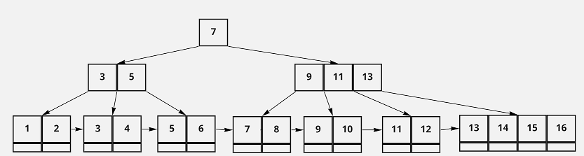
Note that the actual data for the Employee relation would be stored in the leaf nodes of the above tree.
-
Let’s say we wanted to do a complete scan of the Employee table’s records. How many disk reads would this scan take?
It would take 9 disk reads. This is because scanning the entire index would mean tracing the B+-tree down to the smallest key, and sequentially reading disk pages from left to right. Each time we follow a reference in the B+-tree, we’d be reading another disk page into memory.Note that even though this is a significant number of disk reads, because each of the pages read is physically contiguous on disk, there would be a far shorter rotational delay in performing the scan, and each disk read would be shorter than an average disk read.
Now let’s say that it’s often useful to lookup an employee’s record by searching by the first name of that employee. If that was the case, we might find it useful to build a secondary index on the firstName field, like so:
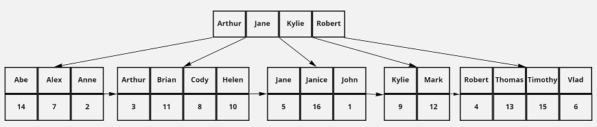
Notice that the keys of this index are the first names of the employees, and the values are that employee’s id.
-
How many disk reads would it take to search for all Employee records where the employee’s first name is Timothy, leveraging both indices?
Using both the secondary and the primary indices, it would take 5 total disk reads. This is because we have to read 2 pages into memory as we search the secondary index for Timothy’s key. Once we find it, we can use its value (15) as our search key in the primary index. Searching the primary index for id 15 requires 3 more reads. Thus, the search cost us 5 disk reads overall. -
How many disk reads would the same search take if you were limited to just the primary index?
If we could only use the primary index, we would have no choice but to scan the entire index for Timothy’s name, reading each page into memory and looking for a firstName field equal to “Timothy”. Since the primary index isn’t ordered by firstName field, we’d have to scan all pages before we could safely say we’d found all employees with the first name “Timothy”. Per the previous question, a full scan of the primary index would take 9 disk reads.
Tuning Database Indices
-
When is it a good idea to add a secondary index to your table?
When SELECT queries are running slowly, especially those involving non-primary key fields. -
When is it a good idea to remove a secondary index from your table?
When UPDATE queries are running slowly against your database. -
How does removing a secondary index speed up UPDATEs?
Updates need to be propagated against all indices. That means that, with multiple indices, a single update can result in a large number of changes to different indices.
Last updated on December 5, 2024.